R comes with a plethora of data sets to play with out of the box, which really come in handy when you're exploring how new functions work. While Python's pandas package tries to emulate the best parts of R's data frames, it can be tedious to find "real world" data sets to load or try to create your own toy data sets. Well, thanks to the rpy2 package (and some incredibly arcane code snippet that will likely change in the future) you can import any of R's data sets directly into a pandas data frame!

The rpy2 package itself is actually quite a gem. If you have R 3.0+ installed in your environment, rpy2 provides an interface to execute R code from python and interact with the results as if they were python objects. This makes rpy2 like a super-library that lets one use some of the best parts of R from python. I haven't dared try anything too complicated with rpy2 just yet, but I knew if I could just get R's data sets into a pandas data frame that I'd end up using them. Take a look at all the data sets at your fingertips in R: (https://stat.ethz.ch/R-manual/R-patched/library/datasets/html/00Index.html)

If you'd like to inspect the data sets from R itself:

# Start R interpreter from bash
$ R
# Interactively look at what data sets are available
> data()
# Data sets in package ‘datasets’:
# 
# AirPassengers           Monthly Airline Passenger Numbers 1949-1960
# BJsales                 Sales Data with Leading Indicator
# BJsales.lead (BJsales)
#                         Sales Data with Leading Indicator
# BOD                     Biochemical Oxygen Demand
# ...
# volcano                 Topographic Information on Auckland's Maunga
#                         Whau Volcano
# warpbreaks              The Number of Breaks in Yarn during Weaving
# women                   Average Heights and Weights for American Women

# Let's look at the BOD data
> BOD
#   Time demand
# 1    1    8.3
# 2    2   10.3
# 3    3   19.0
# 4    4   16.0
# 5    5   15.6
# 6    7   19.8

# Use the R Help to to view the description, the source, and some examples
> ?BOD

# Summarize it from R
> summary(BOD)
#      Time           demand
# Min.   :1.000   Min.   : 8.30
# 1st Qu.:2.250   1st Qu.:11.62
# Median :3.500   Median :15.80
# Mean   :3.667   Mean   :14.83
# 3rd Qu.:4.750   3rd Qu.:18.25
# Max.   :7.000   Max.   :19.80

# Let's look at the AirPassengers data set, too
> AirPassengers
#      Jan Feb Mar Apr May Jun Jul Aug Sep Oct Nov Dec
# 1949 112 118 132 129 121 135 148 148 136 119 104 118
# 1950 115 126 141 135 125 149 170 170 158 133 114 140
# 1951 145 150 178 163 172 178 199 199 184 162 146 166
# 1952 171 180 193 181 183 218 230 242 209 191 172 194
# 1953 196 196 236 235 229 243 264 272 237 211 180 201
# 1954 204 188 235 227 234 264 302 293 259 229 203 229
# 1955 242 233 267 269 270 315 364 347 312 274 237 278
# 1956 284 277 317 313 318 374 413 405 355 306 271 306
# 1957 315 301 356 348 355 422 465 467 404 347 305 336
# 1958 340 318 362 348 363 435 491 505 404 359 310 337
# 1959 360 342 406 396 420 472 548 559 463 407 362 405
# 1960 417 391 419 461 472 535 622 606 508 461 390 432
> quit()

Now let's get that data into Python. Note that here, I'm using pandas 0.17.x and I'm following the related documentation. As of 0.17.0 there appears to be a deprecated interface to rpy (predecessor to rpy2) in pandas that's much cleaner to use, but not future-proof. I will use the (ugly) supported version and expect that this will become cleaner in later versions of pandas.

## Arcane incantation
>>> from rpy2.robjects import pandas2ri
>>> pandas2ri.activate()
>>> from rpy2.robjects import r

# Now, provide your data set name to the r object
>>> df_BOD = pandas2ri.ri2py(r['BOD'])
>>> df_BOD
#    Time  demand
# 1     1     8.3
# 2     2    10.3
# 3     3    19.0
# 4     4    16.0
# 5     5    15.6
# 6     7    19.8

>>> df_BOD.info()
# <class 'pandas.core.frame.DataFrame'>
# Int64Index: 6 entries, 1 to 6
# Data columns (total 2 columns):
# Time      6 non-null float64
# demand    6 non-null float64
# dtypes: float64(2)
# memory usage: 144.0 bytes

# Note that some of these data sets are not 

This works pretty well for converting R data frames into pandas data frames. Some data structures are a little trickier to convert, like R "time series"

>>> df_AP = pandas2ri.ri2py(r['AirPassengers'])
>>> df_AP
# array([ 112.,  118.,  132.,  129.,  121.,  135.,  148.,  148.,  136.,
#         119.,  104.,  118.,  115.,  126.,  141.,  135.,  125.,  149.,
#         170.,  170.,  158.,  133.,  114.,  140.,  145.,  150.,  178.,
#         163.,  172.,  178.,  199.,  199.,  184.,  162.,  146.,  166.,
#         171.,  180.,  193.,  181.,  183.,  218.,  230.,  242.,  209.,
#         191.,  172.,  194.,  196.,  196.,  236.,  235.,  229.,  243.,
#         264.,  272.,  237.,  211.,  180.,  201.,  204.,  188.,  235.,
#         227.,  234.,  264.,  302.,  293.,  259.,  229.,  203.,  229.,
#         242.,  233.,  267.,  269.,  270.,  315.,  364.,  347.,  312.,
#         274.,  237.,  278.,  284.,  277.,  317.,  313.,  318.,  374.,
#         413.,  405.,  355.,  306.,  271.,  306.,  315.,  301.,  356.,
#         348.,  355.,  422.,  465.,  467.,  404.,  347.,  305.,  336.,
#         340.,  318.,  362.,  348.,  363.,  435.,  491.,  505.,  404.,
#         359.,  310.,  337.,  360.,  342.,  406.,  396.,  420.,  472.,
#         548.,  559.,  463.,  407.,  362.,  405.,  417.,  391.,  419.,
#         461.,  472.,  535.,  622.,  606.,  508.,  461.,  390.,  432.])

Note: in R our "time series" object appears to have column names (months) and row names (years). These fields are not readily available to use as attributes in either R or python. In R the row names are internally represented by time series attributes with start=1949, end=1960, frequency=12.

On the first day of the new year, I suffered the loss of my 3.5 year-old Macbook Air and quickly set out to find a replacement. I ultimately settled on a 13" Macbook Pro with Retina Display. From my previous workhorse, I've doubled my memory and SSD storage to 8GB and 250GB, respectively, without noticing the slight weight increase.

Getting up and running on a new machine can be an arduous task, so I've taken some notes on what I ultimately needed. Note that some of these installs (e.g. Slate) may come from third-party developers or require some sort of privileged access that requires fiddling with some settings to enable. Two places to remember are System Preferences -> General (Toggle to "Allow apps from Anywhere" temporarily), System Preferences -> Privacy -> Accessibility (Toggle which apps can "control your computer").

OS and GUI applications

• Open the App Store
• First thing, upgrade OS if applicable (in my case, Yosemite to El Capitan)
• Install XCode from the App Store
• Install Evernote from the App Store, while we're at it.
• Install Alfred from the App store, too.
• Install Caffeine.
• Chrome - because Safari just won't do.
• Firefox - when Chrome isn't supported.
• XQuartz - for GUIs
• Spotify - for music
• f.lux - so I can sleep at night
• iTerm2 - my preferred terminal
• Rescuetime "Lite" - Note: log in first, then download rescuetime to track your device
• Virtualbox - I like to target Ubuntu environments
• Dropbox - for file sharing
• Hipchat - work chat

Command Line installs

Now we're getting into the command line configuration

Homebrew installs

• Homebrew
• After installing homebrew, you may need to restore permissions: sudo chown -R $(whoami) /usr/local

brew install r
brew install git
brew install htop-osx
brew install openssh
brew install readline
brew install sqlite
brew install tmux
brew install tree
brew install wget
brew install vagrant

Misc

• Install my dotfiles git clone https://github.com/tyleraland/dotfiles.git && bash dotfiles/install.sh
• Slate is a fantastic tool for window management in OSX with keyboard shortcuts. I use CMD+CTRL+X, where X is a key easily within reach. I use slate for summoning frequently used applications, hiding windows, resizing windows, and moving windows. Note you'll need to allow Slate to "control your computer", as described above.
• sshfs - for mounting remote filesystems using the SSH protocol

wget http://sourceforge.net/projects/osxfuse/files/osxfuse-2.8.2/osxfuse-2.8.2.dmg && open osxfuse-2.8.2.dmg
wget https://github.com/osxfuse/sshfs/releases/download/osxfuse-sshfs-2.5.0/sshfs-2.5.0.pkg && open sshfs-2.5.0.pkg

Note: On my remote filesystem, I want to access files that are not owned by me but are controlled by groups that are not defined locally on my Mac. As a result, I get "Permission Denied". The solution I've found to this problem is to add those groups to my local mac and add my local user to those groups, like so:

$ sudo dseditgroup -o create -i $REMOTEGID $REMOTEGROUP # Create the group
$ sudo dseditgroup -o edit -a $(whoami) -t user $REMOTEGROUP # Append my user name to the group definition

Python Installs

With homebrew + python, don't make the mistake of using sudo. The result will be initial success, but files will ultimately be owned by root (and not your user). This may be what you want, but you may also have issues down the road. You can chown -R $(whoami) /usr/local to attempt to reset ownership. Failing that (as in my case), you can sudo pip uninstall your packages and attempt to re-install without sudo.

brew install python --with-berkeley-db4 --with-tcl-tk # python >= 2.7.11
pip install -U pip
pip install -U setuptools
pip install -U virtualenv
# Scientific python stack
pip install numpy
pip install pandas
pip install scipy
pip install matplotlib
pip install ipython
# Misc
pip install beautifulsoup4
pip install ghp-import
pip install jinja2
pip install Markdown
pip install markdown2
pip install pelican
pip install scons
pip install jupyter
pip install csvkit
pip install ansible

Systems settings

• Map Caps Lock to CTRL: System Preferences -> Keyboard -> Keyboard -> Modifier Keys ->

Java

• Download and install Java SDK
• Download and install Eclipse SDK

Thanks

Lots of thanks to my boss Noah Hoffman for his (very similar) blog post.

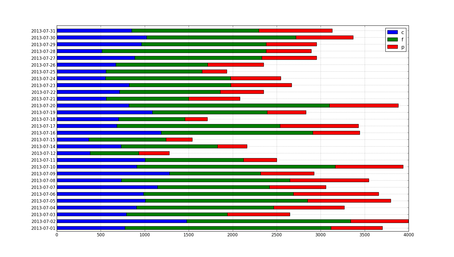
After much data collection and munging, I'm proud to present this graph of my strange eating habits for July 2013. This breaks down my caloric consumption for each day by carbohydrates (blue), fat (green), and protein (red). I have data from March 2013 through August 2013, but I chose to drill down on just July. In this month, I'd been experimenting with high-fat, low-carbohydrate/ketogenic diets for about 12 months and meticulously logging my food consumption, among other things. By July, the experiment was over and I'd begun to consciously increase my carbohydrate intake, so it should look a little more "balanced" than prior low-carb months.

Here are some of my observations using python's 'pandas' library:

# 'd' is a pandas.DataFrame of Calories by Carbs,Fat,Protein

print(d)
# 2013-07-01 773.4620 2344.1805 583.7460
# 2013-07-02 1477.0428 1862.5788 656.9180
# 2013-07-03 791.2992 1145.7504 712.7120
# 2013-07-04 907.0984 1559.7909 801.1384
# 2013-07-05 1006.6896 1843.2441 947.5256
# 2013-07-06 986.8680 1703.7360 967.3420
# 2013-07-07 1143.6960 1274.3370 641.9880
# 2013-07-08 732.8176 1916.7201 896.9908
# 2013-07-09 1281.9548 1033.5897 607.8372
# 2013-07-10 910.2628 2255.0328 772.5288
# 2013-07-11 1004.7800 1116.3654 380.2240
# 2013-07-12 377.8120 552.9510 347.5000
# 2013-07-14 730.3320 1097.0370 335.5200
# 2013-07-15 363.4920 878.4405 297.7760
# 2013-07-16 1185.7132 1724.7879 533.2016
# 2013-07-17 683.2420 1853.9460 891.6680
# 2013-07-18 701.2500 755.7300 255.1960
# 2013-07-19 1086.4212 1304.2854 443.5876
# 2013-07-20 820.5680 2279.5200 781.1020
# 2013-07-21 562.9880 935.3340 582.4880
# 2013-07-22 713.1772 1146.1482 491.8272
# 2013-07-23 822.6144 1156.8348 690.3592
# 2013-07-24 553.5544 1421.2611 570.9420
# 2013-07-25 558.5900 1093.3965 282.0560
# 2013-07-26 671.7104 1042.0452 636.4024
# 2013-07-27 885.8336 1445.3289 622.4760
# 2013-07-28 511.8304 1867.7844 512.1832
# 2013-07-29 963.0200 1416.5055 572.4840
# 2013-07-30 1019.4208 1697.9346 650.9468
# 2013-07-31 850.8284 1446.4989 832.9432

One of the first things I was curious to investigate was my macronutrient ratios.

# Total monthly Calories of [Carb, Fat, Protein]
totalc = map( lambda k: int(pandas.np.sum(d[k])), d.keys())

# Daily average in grams
totalc[0] / 4 / len(d) # 4 Calories per gram of carbohydrate
totalc[1] / 9 / len(d) # 9 Calories per gram of fat
totalc[2] / 4 / len(d) # 4 Calories per gram of protein
# 208g Carb
# 159g Fat
# 152g Protein
# 208g Carbohydrate

# Ratios
map( lambda nut: float(nut)/pandas.np.sum(totalc), totalc)
# 29% Carbohydrate
# 50% Fat
# 21% Protein

First, but not most surprisingly, I'm eating many more carbohydrates (208g) than my previously ketogenic diet would permit. With that said, I've had plenty of energy. I've been weightlifting regularly (July was a very consistent month) and as I've increased my carbohydrates and decreased my fat, I've been steadily gaining muscle as well as fat.

Second, I manage to eat a staggering amount of fat! When I was tracking my food, I was concerned my fat intake would appear low because of how difficult it is to track cooking oil consumption--not so, apparently. With 50% of my Calories coming from fat (predominantly monounsaturated and saturated, I'll bet), I'm well above the USDA's upper-recommendations of 30%, which makes me quite the deviant.

Third, I have been shooting for 150-200g protein per day. I'm just barely meeting my goal at 150g. This is a little annoying to me, but it looks to be low because of the occasional low-protein day. July was a great month for muscle gain, so I can't complain too much. This data is missing several foods that I had issues tracking (protein powder) because they weren't in the easy database.

pandas.np.sum(totalc) / len(d)
# 2884

Lastly, my caloric intake is all over the place. 2880 Calories is roughly the intake I've been shooting for to gain muscle and maintain fat, but my lowest-Calorie day is about 1/3 my highest-Calorie day. This may be due to a data error ... I'll have to investigate later.

As for the data I've been collecting, this is the tip of the iceberg. In the future I plan on looking at how my macronutrient ratios have changed month-to-month, what I eat, what kinds of vitamins/minerals I get, my meal frequency, and many more fun observations.

Around March 2013, I began tracking the food that I eat, logging workouts, and taking miscellaneous personal notes with Twitter. At first, my goals were simple: start tracking as much as possible and then analyze it later. Over time, I settled on tracking food consumption, workouts, and mood. My hypothesis (biases aside) is that the food that I eat and the exercise that I do has a measurable effect on my quality of life.

Before I settled on logging with Twitter, I shopped around for other tracking apps for my Android phone, but wasn't satisfied with how the app addressed my use case. Particularly for food: what if the food I eat isn't in the database? How long does it take me to open the app, type in the food, use the drop-down, select a quantity and units? I contemplated writing my own Android app to ease these concerns, but fortunately settled on a stupidly simple semi-structured text solution using Twitter.

I learned of a Google Apps Script that I could run, free of charge, on a daily timer, to copy my Twitter archive to Google Drive. With all my data in one places, I could parse the data with python into rows keyed by timestamp and containing text for tokenizing and analysis.

At first, I had doubts that I could habitually track all of my food without developing some neuroses. The data, actually, was straightforward to collect and had some positive side effects on my behavior. The practice helped be much more mindful about the food that I eat, what ingredients are in my food, how that food makes me feel, etc. I'd find myself declining to eat something because it wasn't worth the effort to track it.

When logging food, I use an abbreviation for the particular food that I'm eating that's defined in a text file. That abbreviation is mapped to entries in the USDA National Nutrient Database, a giant table with >8,000 rows of foods and measurements of 140 nutrients found in those foods, including macronutrients, individual fatty acids, individual amino acids, vitamins, and minerals.

The parsing-and-analysis step is an ongoing hack-fest, but I will be committing over on Github. My new revised goal for this project is to build a (personal) platform for logging everything possible with semi-structured text. I don't intend for this code to be meaningful to anyone but me, but maybe it will enable some interesting analyses to share!

Today I'll share some of the goodies I've found while exploring scikit-learn's tutorial and practice embedding code snippets in posts. I'll try to avoid just rehashing the tutorial. To get started, scikit-learn (and numpy, which it depends on) should be installed. I also assume we're using ipython, since it makes exploring objects more fun. Any '?' or '%' prefixes to the following code snippets are functions of IPython.

from sklearn.datasets import load_iris
iris = load_iris()

The iris dataset is commonly used among the Machine-Learning/Data-Mining communities. Enough is known about the properties of the data that practitioners are confident using it as a test case for new algorithms and the like. I like that it comes built in! To start, let's pretend we don't know anything about the iris data.

iris?              # Not helpful--whhat attributes are available?
iris.         # .DESCR, .data, .target, feature_names ...
print(iris.DESCR)  # Data summary, features and classes...
iris.data?         # Ah, a numpy ndarray
iris.data.shape    # (data_points, features) == (150, 4)
iris.target        # 1-D array of 0's, 1's, and 2's
iris.target.size   # There are 150; these must be the classes
iris.feature_names # Here is the enumerated type to the 0/1/2's

numpy's arrays are really nice for indexing and slicing.

row, col = 5, 10
iris.data[row]     # Row 5
iris.data[:,col]   # Column 10
iris.data[5,10]    # Element at 5,10
iris.data[[1,2,3]] # Return array of rows 1, 2, and 3
iris.data.argmax() # Largest element in flattened array
iris.data.flatten()[iris.data.argmax()] # 7.9

That was just exploring the data with IPython. If we wanted to completely skip that step, we can jump right in and start learning some rules.

X,y = iris.data, iris.target      # Training set and classes
from sklearn.svm import LinearSVC # Support Vector Classifer
from sklearn.linear_model import LogisticRegression
from sklearn.neighbors import KNeighborsClassifier

# Instantiate each learner
l1 = LinearSVC()
l2 = LogisticRegression()
l3 = KNeighborsClassifier 
new_data =  [[ 5.0, 3.6, 1.3, 0.25]] # Predict its class 

for learner in [l1,l2,l3]:
  learner.fit(X,y)
  print(learner.predict(new_data)) # Each says class-0

I like the standard interface to train and use each classifier. In addition, the LogisticRegression learner also assigns a probability to each possible class.

l2.predict_proba(new_data) # A list of three floats
                           # [.90, ,09, .00]
l2.predict_proba(new_data).sum() # ~ 1.0

Each learner also comes with a "score" method for measuring accuracy relative to provided test and class data. It's straightforward to randomize the data, split it into a 'training' and 'test' set, and compare the learners.

import numpy as np                   # We want to use its arrays
from numpy.random import RandomState # Random functions
RandomState.seed(42)
order = np.arange(0,150)             # Flat array, 0..149

# Shuffle the data, determine the training/testing split
RandomState.shuffle(order)           # Randomize order in situ
X = iris.data[order]
y = iris.target[order]
split = 150 * 2 / 3                  # 2/3 training, 1/3 testing

X_train, X_test = X[:split], X[split:]
y_train, y_test = y[:split], y[split:]

# Now train and test
for learner in l1,l2,l3:
  learner.fit(X_train, y_train)
  print(larner.score(X_test,y_test))

The resulting scores are .92, .88, and .94 respectively. It appears Nearest Neighbors is the champ today.